Introduction
This lesson is focused on how a model forecast and the interpretation of that forecast are affected by the basic design of the model. The content that follows fits under the Dynamics box on the NWP and Weather forecasting chart.
Question 1 of 2
The "model type" refers to whether a model represents meteorological data as point-like (gridpoint) or as a series of waves (spectral), and hydrostatic or nonhydrostatic. Which combination of model types do you think would best be able to explicitly resolve individual thunderstorms?
The correct answer is c.
As we will see shortly, only a non-hydrostatic model can represent the internal pressure gradients and buoyancy effects within a thunderstorm, and hence a) and d) are incorrect. Likewise, spectral models tend to smooth features out too much, such as spreading cold pools. Cold pools often have sharp boundaries, and hence are better represented with gridpoint models with high resolution, and hence b) is incorrect.
Question 2 of 2
The "model type" affects the types of errors the model makes, thus how to interpret the model forecast. See if you can identify some of these influences.
Which of the following are affected by model type? (Choose all that apply.)
The correct answers are a, b, d, e.
Gridpoint and spectral models are based on the same set of primitive equations. However, each type formulates and solves the equations differently. The differences in the basic mathematical formulations contribute to different characteristic errors in model guidance.
The differences in the basic mathematical formulations lead to different methods for representing data. Gridpoint models represent data at discrete, fixed grid points, whereas spectral models use continuous wave functions. Different types and amounts of errors are introduced into the analyses and forecasts due to these differences in data representation.
The characteristics of each model type along with the physical and dynamic approximations in the equations influence the type and scale of features that a model may be able to represent.
Model type does not necessarily impact the size of a model's domain. Global models have historically been spectral because the wave functions and spherical harmonics in the spectral formulation form a natural mathematical basis over a spherical domain, allowing high accuracy in modeling the motion of a fluid on a sphere, such as the atmosphere over the earth. However, global models are increasingly becoming gridpoint as computer resources increase. Nonhydrostatic models are usually limited to small domains because the additional cost of computing the nonhydrostatic terms only helps the forecast of small-scale features requiring high resolution to resolve, and most operational centers don't yet have enough computer power to run a global high-resolution model in real time. However, with increasing computer power, it may only be a matter of time before there are global nonhydrostatic models.
Model type has no direct impact on the choice of horizontal or vertical resolution down to around 10 km horizontal grid spacing. Theoretically, gridpoint and spectral models can be of any resolution, within the limitations of available computing power. However, a model with very fine horizontal resolution should be nonhydrostatic.
After completing this lesson, you will be able to:
- List at least 2 types of weather features which a hydrostatic model of sufficient resolution is not capable of properly predicting because the phenomena are nonhydrostatic in character
- Describe the difference between how a grid point model and a spectral model represent data
- State the primary source of error present in a limited-domain model but not present in a global model, and describe the time evolution of where in the limited-domain model the error appears
- List 2 advantages and 2 limitations of models which use a sigma vertical coordinate or a hybrid which includes sigma coordinates at the bottom of the mode
- State the minimum size feature a gridpoint model can predict well (how many grid boxes wide)
- State at least two impacts of increasing model horizontal resolution on model topography
- State at least two impacts of increasing model horizontal resolution on the resolution of atmospheric features
- State at least 2 types of forecast errors other than temperature errors which occur in complex terrain when the terrain is not adequately resolved
- Describe how the model prediction of boundary layer evolution can be affected by vertical resolution in an area of complex terrain
Hydrostatic vs Non-hydrostatic Models
Hydrostatic vs Non-hydrostatic Models » Hydrostatic Equation
Let's begin by exploring the characteristics and errors associated with gridpoint and spectral models and hydrostatic and nonhydrostatic models in more detail.
Question
The hydrostatic equation is shown above. Which of the following statements best describes its implications? (Choose all that apply.)
The correct answers are b, c, e.
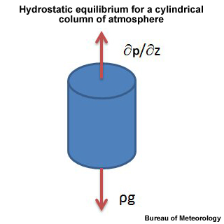
In scaling the vertical momentum equation, it only needs to be shown that Dw/Dt is much smaller than gravity, not zero, hence a) is incorrect. Because there is no term involving time, the equation is only useful for diagnosing the current state of the atmosphere, not for predicting future states, and hence d) is incorrect. Finally, the physical significance of the equation is that the vertical pressure gradient ∂P/∂z is balanced by the weight ρg, which is why we can ignore vertical accelerations, and hence f) is incorrect.
The hydrostatic equation preserves stability within the forecast model and is used to calculate the height field necessary for determining geostrophic balance in the wind forecast equations. This diagnostic equation links the mean temperature in a layer of the model to the difference in height between the upper and lower isobaric surfaces serving as the top and bottom of the layer. Updated temperatures obtained from the temperature forecast equation are used here to calculate heights, which are then used in the wind forecast equations.
Hydrostatic vs Non-hydrostatic Models » Continuity Equation
Vertical motion is calculated using the continuity equation in hydrostatic models. The continuity equation is calculated diagnostically from the horizontal wind fields without considering buoyancy effects. Horizontal divergence is determined from the spatial variations in both of the horizontal wind components. The divergence is then related to the change in vertical motion from the bottom to the top of a layer within the model. Areas of horizontal convergence must coincide either with areas where rising motion increases with height or where sinking motion weakens with height. In pressure coordinates, the vertical motion is omega, Dp/Dt, with omega < 0 associated with ascent. Values of omega are averaged over a grid box, and hence increasing the horizontal resolution will increase the model's ability to resolve fine scale features in omega such as orographic uplift, troughs, cold fronts, etc. It will also result in an increase in the maximum and minimum values observed.

Shown in the figure here is the 850 hPa omega field from the Australian ACCESS model. Purple and orange shades indicate negative values of omega, hence ascent. The field in this case is quite noisy.
Hydrostatic vs Non-hydrostatic Models » Non-hydrostatic Equation
Most nonhydrostatic models use gridpoint formulations. They are generally applied to forecast problems requiring very high horizontal resolution (from tens of meters to a few kilometers) and cover relatively small domains.
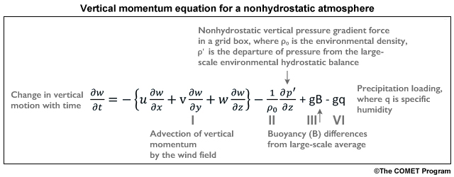
The equation shows that in a nonhydrostatic model, changes in vertical motion may be caused by:
- Orographic uplift or descent (first term)
- Advection bringing in air with a different vertical velocity (first term)
- Pressure deviations from hydrostatic balance resulting from changes in horizontal divergence or phenomena with nonhydrostatic pressure perturbations, such as thunderstorms and mountain waves (second term)
- Buoyancy caused by temperature and or moisture anomalies compared to surrounding grid boxes (third term); g indicates gravity
- Downward drag caused by the weight of liquid or frozen cloud water and precipitation (fourth term)
Most models are hydrostatic, however the Rapid Update Cycle model, or RUC, is fully nonhydrostatic.
Hydrostatic vs Non-hydrostatic Models » Example of Non-hydrostatic Process
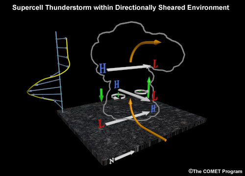
Shown here is an example where a nonhydrostatic model is required to capture the important dynamics and physics. Wind shear within the storm environment gives rise to perturbation pressures within the thunderstorm cell, producing ascent and descent as shown by the green arrows. These perturbation pressure induced circulations give rise to storm splitting.
Question
Match the schematics of various physical processes that occur in the the atmosphere to the appropriate term from the nonhydrostatic vertical momentum equation. Select I, II, III, or IV from the pull-down menu for each schematic.
A shows the internal dynamical pressure gradients within a supercell thunderstorm, where dynamical pressure gradients can produce enhanced updrafts. B shows orographic uplift, involving the vertical advection of vertical gradients of w. Finally, C shows precipitation descending out of the bottom of a thunderstorm, where drag on the air below by the precipitation occurs.
Hydrostatic vs Non-hydrostatic Models » Comparison of Hydrostatic vs Non-hydrostatic
| Hydrostatic | Non-hydrostatic | |
|---|---|---|
| Buoyancy | Indirect (first, horizontal pressure gradients are created, then convergence, finally vertical motion) | Direct (buoyancy - vertical motion) |
| Perturbation pressure acting against buoyancy | No | Yes, important for regulating convective updraft velocity and convective cloud structure and for gravity wave energy propagation |
| Previous vertical motion | No | Yes, vertical motion is advected |
| Water loading | No | Yes |
Question
The hydrostatic approximation only applies well to phenomena which have a longer horizontal length (L) than vertical depth (D). Which of the following phenomena would require a nonhydrostatic treatment?
The correct answers are c, d, e, f.
Fronts are often very long and slope with height. Likewise, the sea breeze front is quite shallow. Hence a) and b) are incorrect. Weak diabatic forcing means that the resulting buoyancy forces are weak and hence g) is incorrect.
Boundary layer rolls involve buoyancy forcing from surface heating. Tropical cyclone eye walls typically contain intense deep convection. Intense latent heating is associated with buoyancy generation, and microphysical feedbacks produce latent heating or cooling.
Gridpoint vs Spectral Data Representation
Grid Point Representation
Shown here is a representation of a temperature field by a gridpoint model, in degrees Celsius.
Question 1 of 2
Instructions: Using the pen tool, analyse the field by drawing isotherms at 2°C intervals, beginning at 0°C.
| Tool: | Tool Size: | Color: |
|---|---|---|
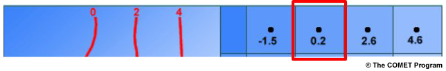
In the real atmosphere, temperature, pressure, wind, and moisture vary from location to location in a smooth, continuous way. In the graphic, the continuous temperature field is depicted with the red contours, labeled in degrees Celsius. Gridpoint models, however, perform their calculations on a fixed array of spatially disconnected grid points. The values at the grid points actually represent an area average over a grid box. The continuous temperature field, therefore, must be represented by grid boxes of fixed temperature, indicated by the shades of blue in the right panel, each identified by a single gridpoint value as shown by the black numbers.
Question 2 of 2
Derivatives in the forecast equations are approximated using finite differences. Calculate the derivative for the box indicated and answer the following questions.
The gradient is steeper to the east, being (2.6 – 0.2)/Δx = 2.4/Δx compared to (0.2 - -1.5)/Δx = 1.7/Δx.
Finite differencing smooths out the gradient, giving (2.6 - -1.5)/2Δx = 2.05/Δx. This represents a loss of information.
Gridpoint vs Spectral Data Representation » Grid Cubes
Gridpoint models actually represent the atmosphere in three-dimensional grid cubes, such as the one shown. The temperature, pressure, and moisture (T, p, and q), shown in the center of the cube, represent the average conditions throughout the cube. Likewise, the east-west winds (u) and the north-south winds (v), located at the sides of the cube, represent the average of the wind components between the center of this cube and the adjacent cubes. Similarly, the vertical motion (w) is represented on the upper and lower faces of the cube.
This arrangement of variables within and around the grid cube (called a staggered grid) has advantages when calculating derivatives. It is also physically intuitive; average thermodynamic properties inside the grid cube are represented at the center, while the winds on the faces are associated with fluxes into and out of the cube. Different models employ different staggered grid arrangements. Model output is interpolated vertically and horizontally to a common grid during postprocessing.
Gridpoint vs Spectral Data Representation » Spectral Data Representation
Spectral models represent the spatial variations of meteorological variables (such as geopotential heights) as a finite series of waves of differing wavelengths.
Shown here is hemispheric 500-hPa height field. The green circle is 40° N and the yellow dots are 10° of longitude apart, so there are 36 points around the globe. It takes a minimum of five to seven points to reasonably represent a wave and, so five or six waves can be defined with the data. The locations of the wave troughs are shown in the top part as solid red lines.
Question 1 of 2
When the 500-hPa height field data are plotted as a wave in the graph in the lower part of the images, the five wave troughs are definable by the white dots but are unequally spaced. What does this indicate?
The correct answer is b.
This indicates the presence of more than one wavelength of small-scale variations. In this case, the shorter waves represent the synoptic-scale features, while the longer waves represent planetary features (planetary waves).
Derivatives in spectral data
Question 2 of 2
Will derivatives in spectral data be smoother or coarser than those for gridpoint data?
The correct answer is a.
Since the forecast variables are represented by continuous analytic functions, horizontal derivatives are represented by the derivatives of these functions with none of the additional loss of accuracy or smoothing that occurs with gridpoint representation.
Gridpoint vs Spectral Data Representation » Forcing in Spectral Models
Spectral models represent meteorological variables using a number of waves, and the "T" number refers to how many waves are used. However, spectral models employ gridpoint representation for calculating forecast variable tendencies in the physics parameterisations. As a result, the forecast variables are transformed back and forth between spectral representation for dynamics calculations and gridpoint representation for physics calculations.
The red line in the graphic illustrates a one-grid-box event, such as latent heating associated with a precipitation bulls eye in a single grid column. The yellow line shows the spectral representation of this event.
Question
The effect of the spectral representation of the latent heating forcing is to
The correct answer is b.
The heating is effectively reduced by 33% in the grid box containing the storm and spread in an oscillating pattern across a wide distance. The example shown is for a maximum wavenumber of T170 (i.e. 170 waves) and a location along 40°N.
The center peak will be higher and the oscillation will taper more quickly with distance as the maximum number of waves is increased, so the artificial effect will be more pronounced at the poorer resolution typical of ensemble members than the single, high-resolution "deterministic" forecast.
Exercises
Exercises » Question 1 of 5
What characteristics of the model forecast equations limit the accuracy of the forecast? (Choose all that apply.)
The correct answers are a, b.
The equations are limited by approximations made to the physics terms and by the mathematical methods used to derive the equations, which result in approximations to their solutions, even if the initial values for the terms are accurately determined. The accuracy of the solutions to the model forecast equations directly impacts the forecast model output. The equations can be solved accurately, especially in higher resolution models using spectral methods.
Exercises » Question 2 of 5
What does the use of gridpoint or spectral methods enable NWP models to do? (Choose all that apply.)
The correct answers are b, d.
A finite representation of the full atmosphere and mathematical framework are necessary to perform the calculations of the model equations. However, both methods lead to incomplete representation of the atmosphere due to approximations within the model equations and in the methods used to solve them. Hence, completely accurate solutions are not possible and calculations in all forecast formulations have errors.
Exercises » Question 3 of 5
Complete the following statements related to the use of each model type. (Use the selection box to choose the best answer that completes the statement.)
To answer this question, one must consider how the fields are represented in each model type. Spectral models use continuous wave functions, whereas grid models use discrete grid boxes to define meteorological fields. The implication of these differences is that spectral models tend to have a better representation of global fields and gradients, while gridpoint models lend themselves to limited-area applications and tend to have a better representation of the effect of physical processes on the evolution of the weather.
Exercises » Question 4 of 5
Complete the following statements that define the primary differences between hydrostatic and nonhydrostatic models. (Use the selection box to choose the best answer that completes the statement.)
The primary difference between hydrostatic and nonhydrostatic models is that nonhydrostatic models can explicitly forecast vertical motion and do not assume hydrostatic balance, as is the case in hydrostatic models.
Nonhydrostatic models have an extra term, which provides a forecast equation for vertical motion. Hydrostatic models do not have a forecast equation for vertical motion and thus cannot be used to simulate convective cells and other phenomena with a depth about the same as their width. If hydrostatic models are run at very high resolution (less than 10 km), they may try to simulate nonhydrostatic events and generate large wind errors and spurious vertical motion fields. Thus, nonhydrostatic models can be useful for forecasting smaller-scale phenomena than can be handled by hydrostatic models.
Nonhydrostatic models are generally applied to forecast problems requiring very high horizontal resolution (from tens of meters to a few kilometers) and therefore cover relatively small domains. Nonhydrostatic computations are costly and provide little advantage in accuracy except at very small scales. As a result, models predicting global scale to synoptic scale phenomena have generally been hydrostatic, though in recent years there has been a trend toward running operational NWP models at high resolution over a large domain.
Exercises » Question 5 of 5
Which model type is best for forecasting each phenomenon described below? (Use the selection box to choose the best answer that completes the statement.)
Global spectral models are the best to use for forecasting the planetary wave pattern for the next seven days and QPF for the next five days. This is due to the fact that spectral formulations allow for real-time integration of the primitive equations over a longer time range than grid point models. In addition, spectral models have global domains that are best for depicting planetary-scale features, while grid point models often have defined boundaries where errors can occur due to inaccurate and inconsistent boundary conditions. A global gridpoint model would also be a good option but was not among the choices available.
Hydrostatic gridpoint models can best forecast synoptic and sub-synoptic phenomena not strongly influenced by buoyancy, such as orographic precipitation, boundary-layer winds, and jet intensity and location. Due to their higher resolution and more detailed representation of topographic features, gridpoint models generally better depict precipitation near terrain.
High-resolution nonhydrostatic models can best forecast the development and evolution of mesoscale convective systems and the propagation of outflow boundaries. Only nonhydrostatic models can explicitly forecast deep convection since they take into account vertical accelerations due to buoyancy. Hydrostatic models can only parameterize convection and cannot represent the thermodynamic processes that occur within deep convection. Nonhydrostatic models are also necessary for modeling flow on scales finer than around 10 km.
Model Type Summary
Model Type Summary » Gridpoint Models
Characteristics
- Data are represented on a fixed set of grid points
- Resolution is a function of the gridpoint spacing
- All calculations are performed at grid points
- Finite difference approximations are used for solving the derivatives of the model's equations
- Error is introduced through finite difference approximations of the primitive equations
- The amount of error is a function of grid spacing and time-step interval
Disadvantages
- Finite difference approximations of model equations introduce a significant amount of error
- Small-scale noise accumulates when equations are integrated for long periods
- The magnitude of computational errors is generally more than in spectral models of comparable resolution
- Boundary condition errors can propagate into regional models and affect forecast skill
Advantages
- Can provide high horizontal resolution for regional and mesoscale applications
- Do not need to transform physics calculations to and from gridded space
- As the physics in operational models becomes more complex, grid point models are becoming computationally competitive with spectral models
- Nonhydrostatic versions can explicitly forecast details of convection, given sufficient resolution and detail in the initial conditions
Models
- UMKO, ACCESS suite of models.
Model Type Summary » Spectral Models
Characteristics
- Data are represented by wave functions
- Resolution is a function of the number of waves used in the model
- Model resolution is limited by the maximum number of waves
- The linear quantities of the equations of motion can be calculated without introducing computational error
- Grids are used to perform non-linear and physical calculations
- Transformations occur between spectral and gridpoint space
- Equations can be integrated for large time steps and long periods of time
- Originally designed for global domains
Disadvantages
- Transformations between spectral and gridpoint physics calculations introduce errors in the model solution
- Generally not designed for higher resolution regional and mesoscale applications
- Computational savings decrease as the physical realism of the model increases
Advantages
- The magnitude of computational errors in dynamics calculations is generally less than in gridpoint models of comparable resolution
- Can calculate the linear quantities of the equations of motion exactly
- At horizontal resolutions typically required for global models, spectral models require less computing resources than gridpoint models with equivalent horizontal resolution and physical processes
Models
- ECMWF, US GFS, JMA and CMC models
Model Type Summary » Hydrostatic Models
Characteristics
- Use the hydrostatic primitive equations, diagnosing vertical motion from predicted horizontal motions
- Used for forecasting synoptic-scale phenomena, can forecast some mesoscale phenomena
- Used in both spectral and gridpoint models
Disadvantages
- Cannot predict vertical accelerations
- Cannot predict details of small-scale processes associated with buoyancy
Advantages
- Can run quickly over limited-area domains, providing forecasts in time for operational use
- The hydrostatic assumption is valid for many synoptic- and sub-synoptic-scale phenomena
Models
- All global and regional scale models
Model Type Summary » Non-hydrostatic Models
Characteristics
- Use the nonhydrostatic primitive equations, directly forecasting vertical motion
- Used for forecasting small-scale phenomena
- Predict realistic-looking, detailed mesoscale structure and consistent impact on surrounding weather, resulting in either superior local forecasts (sometimes) or large errors (other times)
Disadvantages
- Take longer to run than hydrostatic models with the same resolution and domain size
- Used for limited-area applications, so they require boundary conditions (BCs) from another model; if the BCs lack the structure and resolution characteristic of fields developing inside the model domain, they may exert adverse influence on the forecast
- May predict realistic-looking phenomena, but the timing and placement may be unreliable
Advantages
- Calculate vertical motion explicitly
- Explicitly predict release of buoyancy
- Account for cloud and precipitation processes and their contribution to vertical motions
- Capable of predicting convection and mountain waves
Models
- RUC, WRF
Vertical Coordinates
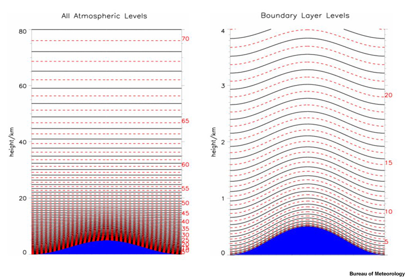
A model's vertical structure is as important in defining the model's behavior as the horizontal configuration and model type. Proper depiction of the vertical structure of the atmosphere requires selection of an appropriate vertical coordinate and sufficient vertical resolution. Virtually all operational models use discrete vertical structures. As such, they produce forecasts for the average over an atmospheric layer between the vertical-coordinate surfaces, not on the surfaces themselves.
Question
Shown in the figure is an idealised surface profile. What kind of properties should a vertical coordinate system have?
The coordinate system should:
In choosing a vertical coordinate system for a numerical model, the coordinate
- Should preserve conservative atmospheric properties and treat important dynamical processes accurately, such as adiabatic and diabatic motion and flow over terrain
- Must exhibit monotonic behavior with height such that the coordinate system does not appear at several levels
- Should accurately represent the pressure gradient force over both flat and sloping terrain
- It shouldn't intersect the earth or pressure levels near the surface
Vertical Coordinates » Sigma Coordinates
Pressure coordinate systems are not particularly suited to solving the forecast equations because they can intersect mountains and consequently 'disappear' over parts of the forecast domain. In order to solve this problem, the sigma coordinate is terrain following.
The sigma coordinate is defined by σ = p/ps, where p is the pressure on a forecast level within the model and ps is the pressure at the earth's surface, not mean sea level pressure. The lowest coordinate surface (usually labeled σ = 1) follows a smoothed version of the actual terrain. Note that the terrain slopes used in sigma models are always smoothed to some degree. The other sigma surfaces gradually transition from being nearly parallel to the smoothed terrain at the bottom of the model (σ = 1) to being nearly horizontal to the constant pressure surface at the top of the model (σ = 0). The top layer of the model is typically placed well above the tropopause.
Vertical Coordinates » Sigma Coordinates » Advantages of Sigma Coordinates
Four advantages of the sigma coordinate are listed below. Some have questions for you to answer.
Advantage #1: Since the sigma coordinate is related to pressure, it produces relatively simple formulations for handling the lower boundary without overly complicating the equations of motion. The simplified formulations are easier to program.
Advantage #2: The sigma coordinate conforms to naturally sloping terrain.
Question 1 of 3
What types of phenomena does this enable the sigma coordinate models to predict? (Select all the apply.)
The correct answers are a, c.
The terrain-following nature of the sigma coordinate allows for good depiction of continuous fields, such as temperature advection and winds, especially in areas where terrain varies widely but smoothly. Additionally, the sigma coordinate can predict such phenomena as downslope wind events in the lee of mountain slopes. However, since the coordinate allows for continuous flow over mountains, it can have difficulty forecasting situations where the mountains act as barriers to flow, for example, cold-air damming in the lee of mountains and leeside cyclogenesis.
Advantage #3: The terrain-following nature of the sigma coordinate lends itself to increasing vertical resolution near the ground consistently over the full model domain.
Question 2 of 3
What is the advantage of having higher resolution in the lower atmosphere? (Select True or False for each statement.)
The model can better define boundary-layer processes and features that contribute significantly to sensible weather elements, such as diurnal heating, low-level winds, turbulence, low-level moisture, and static stability.
Advantage #4: Unlike pressure, height, or isentropic coordinates, the sigma coordinate eliminates the problem of vertical coordinate surfaces intersecting the ground. The other coordinate systems can intersect with the earth's surface in areas of uneven terrain or in areas with strong variation in surface pressure across weather systems.
Question 3 of 3
Meteorologically, why is it a problem when vertical model surfaces intersect the ground? (Type your response in the box below.)
When a model layer intersects the ground, the wind field (and thus temperature and moisture advection) in the area can be interrupted or blocked, which is physically incorrect. To compensate for this error, sophisticated mathematical techniques must be used in the model.
Vertical Coordinates » Sigma Coordinates » Limitations of Sigma Coordinates
Sigma coordinates face limitations in the presence of steep topography
Limitation #1: Sloping sigma surfaces complicate the calculation of the pressure gradient force, which can introduce substantial errors in wind forecasts.
Question 1 of 2
Which of the following statements best describes the limits of representing flow over strongly sloping terrain in a model using sigma coordinates?
The correct answer is b.
To calculate a PGF in a sigma model, we must determine an equivalent to the z1 and z2 on the pressure surface. However, because the sigma model produces data only along sigma coordinate surfaces, it has values at z3 and z4. Two additional terms shown in the graphic are needed to convert the heights on the sigma surface to corresponding heights on the pressure surface. This introduces error. To determine the height difference on the sigma surface corresponding to the z2 - z1, we must take the difference between the height difference along the sigma surface (z4 - z3) and the correction term (z2 - z4) + (z3 - z1), both parts of which depend upon the approximated lapse rate between the sigma surfaces. Both of these terms are much larger than the height difference on the pressure surface, and the resulting difference in the terms can lead to significant errors. The larger the slope of the sigma surface, such as in the green area, the larger the possible error in the PGF.
Limitation #2: Because the actual and often abrupt steepness of mountain slopes is smoothed in sigma coordinate models, they often misrepresent the true surface elevation. This smoothing will particularly affect topography near coastlines.
Question 2 of 2
What impacts might this smoothing of topography have on model output for mountain slopes and ranges near oceanic coasts? (Type your response in the box below.)
The abrupt steepness of mountain slopes can cause forecasts for locations immediately adjacent to mountain ranges to severely misrepresent the surface pressure and thus the temperature and moisture.
Likewise, the smoothing required in mountain ranges along oceanic coasts, land points in the model can be forced to extend beyond the true coastline. Values of temperature and moisture will be different from their true, maritime values.
Vertical Coordinates » Sigma Coordinates » More Limitations of Sigma Coordinates
Sigma models can have difficulty dealing with weather events in the lee of mountains, for example, cold-air damming and leeside cyclogenesis.
In strong cold-air damming events, the inversion (vertical temperature gradient) in the real atmosphere above the cold air mass, shown in the right portion of the figure, is transformed in part into a "horizontal" temperature gradient along the steeply sloped sigma surfaces. As a result, the model can move the cold air away from the mountains through "horizontal" advection along the sigma surfaces, rather than channeling the flow over the mountains above and parallel to the inversion above the cold air.
Likewise, excessive low-level downslope flow means that air parcels on the lowest sigma level will descend further than they would in the real atmosphere, resulting in exaggerated "vortex-tube stretching" of the atmospheric column. This can produce exaggerated and too-frequent leeside cyclogenesis via the generation of cyclonic vorticity.
Vertical Coordinates » Hybrid coordinates
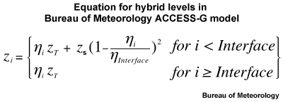
Hybrid vertical coordinate systems combine two coordinate system in a seamless manner, between terrain following coordinates near the surface to constant geopotential surfaces in the upper atmosphere. The levels and related equations shown are for the ACCESS model, where zi is the geopotential height above mean sea level of model level i, zT is the geopotential height at the top of the model, zS is the terrain height above mean sea level, ηi is the "eta" value of model level i and ηInterface is the "rho"-level η value at i = Interface.
Models like the ECMWF use sigma and pressure levels.
Vertical Coordinates » Hybrid Isentrope-sigma Coordinates

Some other models use a sigma level and isentropic or potential temperature coordinate system. Because of problems with the boundary layer typically being non-adiabatic, isentropic coordinates must be used in a hybrid system.
The boundary sigma layer must be sufficiently deep to be able to model diurnal boundary-layer processes, including friction and heating. This typically requires that the sigma boundary layer be approximately 200 hPa deep. If the sigma layer is too shallow, superadiabatic layers can still form or will not be treated properly above the boundary sigma domain.
Question 1 of 2
Match each vertical coordinate system to its primary advantage in NWP models for depicting weather. (Use the selection box to choose the vertical coordinate system.)
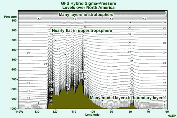
Both sigma and hybrid sigma-pressure coordinates follow model terrain, enabling them to resolve the boundary layer well under all meteorological conditions. However, the hybrid sigma-pressure coordinates are flatter in the middle to upper troposphere and stratosphere above complex terrain, facilitating the assimilation of satellite radiance observations. Flatter coordinates have better numerical properties aloft and improves the efficiency and accuracy of radiative transfer calculations used in assimilating satellite radiance observations. The upper troposphere and stratosphere are crucial for the assimilation of satellite radiance observations, and these observations now play a dominant role in the data assimilation due to their overwhelming abundance.
Just as analyzing data in isentropic coordinates helps the meteorologist to diagnose air streams, moisture, vertical motion, and jet structure in baroclinic environments, isentropic coordinates allow the model to tighten vertical resolution near fronts and jet streaks where the coordinate surfaces are pushed together.
Question 2 of 2
Match each vertical coordinate system to its primary advantage in NWP models for depicting weather. (Use the selection box to choose the vertical coordinate system.)
Both sigma and hybrid sigma-pressure coordinates follow terrain, typically smoothed terrain, resulting in difficulty maintaining cold-air damming while developing lee lows too quickly. Both actually have finer vertical resolution over higher terrain as the same number of model layers are squeezed into a thinner column. Isentropic coordinates cannot handle superadiabatic conditions because then the same potential temperature would appear at two different levels, above and below the superadiabatic layer. Superadiabatic boundary layers are common during the afternoon, so most models employing isentropic coordinates use a hybrid with sigma coordinates in the boundary layer.
Vertical Coordinates » Vertical Coordinates Summary
- All coordinate systems have their strengths and weaknesses
- Most operational NWP models use hybrid coordinates with terrain following coordinates below and pressure surfaces aloft
Advantages
- Sigma
- The terrain-following nature of the sigma coordinate allows for good depiction of continuous fields, such as temperature advection and winds, especially in areas where terrain varies widely but smoothly. Additionally, the sigma coordinate can predict such phenomena as downslope wind events in the lee of mountain slopes.
- Hybrid
- Hybrid vertical coordinate systems combine two coordinate system in a seamless manner, between terrain following coordinates near the surface to constant geopotential surfaces in the upper atmosphere.
- Superadiabatic boundary layers are common during the afternoon, so most models employing isentropic coordinates use a hybrid with sigma coordinates in the boundary layer.
Disadvantages
- Sigma
- Sloping sigma surfaces complicate the calculation of the pressure gradient force, which can introduce substantial errors in wind forecasts.
- Because the actual and often abrupt steepness of mountain slopes is smoothed in sigma coordinate models, they often misrepresent the true surface elevation.
- Sigma coordinates have various problems with steep terrain.
- Hybrid
- If the sigma layer is too shallow, superadiabatic layers can still form or will not be treated properly above the boundary sigma domain.
- Both sigma and hybrid sigma-pressure coordinates follow terrain, typically smoothed terrain, resulting in difficulty maintaining cold-air damming while developing lee lows too quickly.
Model Resolution
Question
Instructions: Using a hypothetical 30-km model (each dot is at the center of a 30x30 km gridbox), assume that a Mesoscale Convective System (MCS) encompasses an area of about > 3000 km2. Identify the echoes associated with the deep convective updrafts with the blue pen. Then with the white pen, indicate the smallest scale feature you think will be properly resolved by the model.
| Tool: | Tool Size: | Color: |
|---|---|---|
The total precipitating area is resolved as indicated in white, because it is represented by 7-8 grid boxes. However, the model cannot adequately resolve the convective updrafts as they are about one grid box. Likewise, all of the physical and microphysical processes embedded in the feature, namely the downdrafts, and other embedded precipitation processes to forecast the MCS's evolution cannot be resolved since these features occur on much smaller scales. The model may initially resolve the feature, but lose it over the forecast period if the physical processes necessary to maintain or develop it cannot be defined.
This means that these processes will need to be parameterized to simulate their effects on the larger-scale environment and their impact on longer-range forecasts.

The obvious solution to a model with poor resolution is to run it at a higher resolution. However, computing resources limit the resolution of NWP models. The additional computing resources required to run a model at half its current horizontal resolution increase by a factor of eight, assuming no change to the vertical resolution or domain size.
Model Resolution » Grid Spacing and Resolution

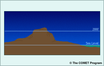
A gridpoint model's horizontal resolution is defined as the average distance between adjacent grid points with the same variables. For example, if all of a model's forecast variables are predicted at each of its grid points, the model is considered to have a resolution equal to the minimum spacing between adjacent grid points at a specific latitude and longitude.
In this example, all of the variables are computed at each grid point so the resolution is 50 km. A similar model with 10 km between adjacent grid points is considered to have 10-km horizontal resolution. However, that does not mean it can resolve features which are only 10 km across!
Question
If the horizontal resolution of a model is increased from 50 km to 10 km, how much will the memory requirements increase by?
The correct answer is c.
The increase in memory is a factor of 5 for an increase in resolution in each horizontal direction, hence 5 x 5 = 25. It is at least this much because a horizontal resolution will typically be accompanied by an increase in vertical resolution, and an increase in timestep.
Model Resolution » Spectral Resolution
In spectral models, the horizontal resolution is designated by a "T" number, which indicates the number of waves used to represent the data. The "T" stands for triangular truncation, which indicates the particular set of waves used by a spectral model.
Spectral models represent data precisely out to a maximum number of waves, but omit all, more detailed information contained in smaller waves. This is in contrast to gridpoint models, which try to represent all scales but poorly handle waves only a few grid points across.
The wavelength of the smallest wave in a spectral model is represented as minimum wavelength = 360 degrees/N
where N is the total number of waves (the "T" number).
For example, a T80 model could resolve a wavelength of 360/80 = 4.5 degrees.
Complications arise because nonlinear dynamics and physics are calculated on a grid and then converted to spectral form to incorporate their effects in a spectral model. This introduces errors, which make the final result less exact than one might expect from calculations done strictly in spectral space.
Question
If the T number of the ECMWF is 1279, what is the minimum wavelength in degrees resolved? Type your answer in the box below.
~0.28°
Model Resolution » Gridpoint Equivalency of Spectral Resolution
It takes about five to seven grid points to get reasonable approximations of most weather features. Still more points per wave feature are often necessary to get a good forecast. Because spectral and gridpoint models preserve information in different ways, no precise equivalent grid spacing can be given for a spectral model resolution.
The approximate grid spacing with the same accuracy as a spectral model can then be represented as ΔX ~ 360° / 3N; where N is the number of waves.

For a T80 model, this results in maximum grid spacing for equivalent accuracy of about 1.5° ~ 160 km (assuming 1° ~ 111 km).
We can approximate the grid spacing to obtain equivalent accuracy to a spectral model with a fixed number of waves using a simple approach. First, we assume that three grid points are sufficient to capture the information contained in each of a series of continuous waves. This is demonstrated by the figure below, where a wavelike feature may be captured by three blue dots to produce the square wave shown, and post processed to the yellow wave.

The dynamics of spectral models retain far better wave representation than gridpoint models with this grid spacing. However, the spectral model physics is calculated on a grid, with about three times as many grid lengths as number of waves used to represent the data. Since it takes five to seven grid points to represent 'wavy' data well and even more for features that include discontinuities, the resolution of the physics is poorer than the above formulation indicates and degrades the quality of the spectral model forecast.
Question
What is the approximate equivalent gridpoint in km for T1279? Assume 1° ~ 111 km. Type your answer in the box below.
DX = 360 / (3 x 1279) ~ 0.09° ~ 0.09 x 111 ~ 10.4 km
Impacts of Model Topography
Two factors that limit model representation of orography are the horizontal resolution of the model and the horizontal resolution of the terrain dataset used.
A model's representation of surface topography is a major factor in its ability to predict meteorological features induced by terrain. The figure shows a realistic topography on the left and a smoothed model topography on the right.
Question 1 of 2
Instructions: If the wind is blowing from left to right in the figure (from the west), use the pen tools to mark in some sample streamlines and regions covered by snow bearing cloud for both the realistic and model topographies.
Hint: because the cloud will be stratiform and orographic, do not draw cloud that is too deep. The key thing to think about here is the resulting horizontal distribution.
| Tool: | Tool Size: | Color: |
|---|---|---|
In the example, windward mountain snow is occurring over a region of steep and complex terrain. Most likely, the model will not be able to predict the precipitation shadow. As a result, the windward clouds and precipitation will be spread over a larger area and will be of less intensity than in reality. The result would be the same either for a coarse-resolution model using a detailed terrain dataset or a fine-resolution model using a coarse terrain dataset.
Why aren't high-resolution gridpoint models run with detailed terrain features at the same scale as the grid spacing? The answer lies in the fact that waves at scales of only a few grid points are poorly represented and even more poorly forecast. Furthermore, as energy in the model accumulates on scales of three or fewer grid points, the computational methods can "blow up" and stop the forecast run prior to completion. Terrain must therefore be smoothed to prevent it from producing such small-scale waves.
Question 2 of 2
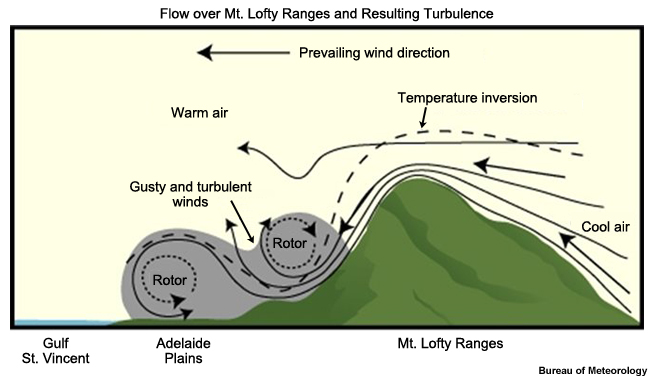
When a strong wind with a significant component perpendicular to mountain ranges occurs underneath an inversion, strong downslope winds with possible rotors and associated turbulence can occur. An example of this is the Adelaide Gully wind.
What impact would a coarse model resolution have on forecast model winds? How would you need to adjust them on both sides of the mountain?
As we saw in the previous question that smoothed model topography is necessary for numerical stability, but will smooth out wind flows and will not resolve downslope winds well and features like rotors (as seen in the image below).
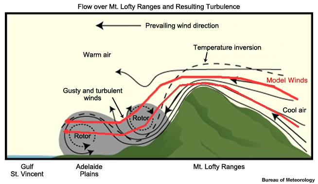
It is likely in these cases that the downslope winds will need to be strengthened, and any aviation products will need to carry moderate to severe turbulence.
Impacts of Model Topography » Model Terrain Impacts
Question
What are some possible effects of inadequate model terrain on weather elements? (Choose all that apply.)
The correct answers are a, c, d, f, g, and h.
In general, insufficient detail in terrain representation impacts a model's ability to forecast terrain-induced and terrain-modified features and processes, and typically not features of the upper troposphere.
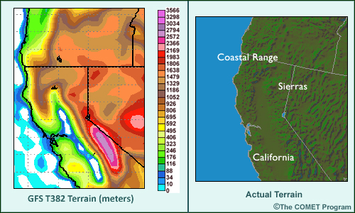
The first graphic below shows the GFS 12- to 36-hr precipitation forecast from 00 UTC 03 March 2009 and the verifying Hydrologic Prediction Center (HPC) analysis. The estimate of observed precipitation and the model forecast have been remapped to the same 32-km grid for comparison. The GFS topography for this region is juxtaposed against a textured topography map in the second graphic below.
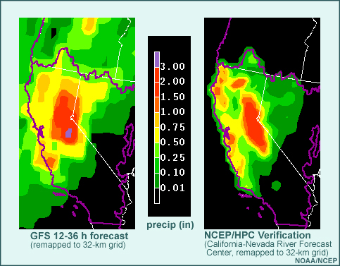
Note these important features:
- Observed precipitation fell primarily over the two mountain ranges
- Model-forecast precipitation maxima extended into the valleys, where little rain actually fell
- Model forecast maximum precipitation amounts were too small along the coastal range in northern California but were similar to the observed maxima in the Sierras. The River Forecast Center estimates of observed precipitation on a much finer grid (not shown) included narrow, elongated patches of 3 to 4 inches.
- Locations of predicted precipitation maxima do not quite line up with the highest terrain or steepest terrain gradients in the model
Gauge reports and fine-scale analyses based on gauge reports will often have larger peak amounts than a model forecast, which represents an average over a grid box (remember, even spectral models calculate precipitation on their transform grid - transforming spectral representations to grid points). An analysis of the observations may even be biased toward higher amounts if gauges are intentionally placed at known wet high-altitude locations, such as for hydrological monitoring.
Impacts of Model Topography » Land/water Interface Considerations
Models also have difficulty resolving features influenced or caused by the interface between land and large bodies of water. This includes oceanic coastal regions and those near the large lakes. Since the properties of land and water are so different, a model will do a poor job of representing the processes that occur or are influenced by land/water interfaces if its resolution is not sufficient to determine their location. For example, models may not place the land/sea interface in the proper location or adequately define its boundary. Smaller lakes are only recognized by very fine-resolution meso- and local-scale models and are not represented in most operational models.
In the example, the coastline in models A and B falls within the purple-shaded regions. In model A, the water/land interface falls within a 40-km band in most areas, the irregularities of the actual coastline are not well represented, and the lake is not recognized at all. In model B, the water/land interface falls within a 20-km band in most places, the actual coastline irregularities are better represented, and three grid points identify the lake.
Question 1 of 2
How will an increase in the model resolution from 40 km to 20 km change how the model will handles sea breezes.
The correct answer is a.
A better resolved land/sea interface will take into account temperature differences across the coastal region, which drive the sea breeze.
Question 2 of 2
How will an increase in the model resolution from 40 km to 20 km most likely change the average summer maximum temperatures at the point marked A?
The correct answer is b.
A better resolution of the sea breeze, will most likely, reduce the daily maximum temperature and hence the average summer temperature.
Impacts of Model Topography » Impact of Feature Size on Resolvability
The relationship between the size of weather features to be predicted and the grid spacing in a gridpoint model is critical. You can see this for yourself in the following exercise.
In this exercise, you will select a weather feature, examine an example of it as described by a wave in a gridpoint model with 20-km resolution, and compare the model to the actual representations of the initial wave and advection of the wave. Many real weather features are asymmetric (such as convection, which has narrow updrafts and broad compensating descent), have sharp edges (such as a dry slot), or are primarily perturbations of one sign (such as surface temperatures associated with an urban heat island). Nonetheless, the same principles related to how well a feature can be represented and maintained in a forecast apply.
As you select and review each weather feature, consider the following questions:
- How many grid points does the wave span?
- Is the gridpoint representation recognizable as a wave-like perturbation?
- Does the model represent the amplitude well?
- If you saw the feature on a satellite or radar loop (shown by the red line) and the model initial fields (plotted like the yellow line), how would you assess the model initial conditions?
- Assuming the feature does not change and is simply advected by perfectly predicted mean flow, how should the model handle the forecast of this feature?
For each example, the complete, initial structure of the weather is represented as a continuous periodic wave (smooth red curve) based on a 20-km model grid. The way in which the model represents the weather feature described by the smooth red curve is shown as a series of blue blocks instead of a smooth curve. These blue blocks represent the average of the actual smooth curve over each grid box. The blue diamonds indicate the grid points located in the center of each grid box. A postprocessed plot of the model gridpoint data would look like the yellow line connecting the gridpoint values, as though the correct values were located at the center of the grid box.
Remember that the gridpoint values represent averages over the entire grid box. In these examples, the initial gridpoint values are exactly equal to the average of the red data curve over the corresponding blue grid box. All deficiencies in representation here result from limitations imposed by resolution.
Impacts of Model Topography » Impact of Feature Size on Resolvability » Urban Smog
The complete, initial structure of the weather is represented as a continuous periodic wave (smooth red curve) based on a 20-km model grid. The way in which the model represents the weather feature described by the smooth red curve is shown as a series of blue blocks instead of a smooth curve. These blue blocks represent the average of the actual smooth curve over each grid box. The blue diamonds indicate the grid points located in the center of each grid box. A postprocessed plot of the model gridpoint data would look like the yellow line connecting the gridpoint values, as though the correct values were located at the center of the grid box.
Remember that the gridpoint values represent averages over the entire grid box. In these examples, the initial gridpoint values are exactly equal to the average of the red data curve over the corresponding blue grid box. All deficiencies in representation here result from limitations imposed by resolution.
The wavelength of this weather feature is ~ 40 kms.
Question 1 of 5
How many grid points does the wave span? Type your answer.
Now answer the next question.
Question 2 of 5
Is the gridpoint representation recognizable as a wave-like perturbation?
Now answer the next question.
Question 3 of 5
Does the model represent the amplitude well?
Now answer the next question.
Question 4 of 5
If you saw the feature on a satellite or radar loop (shown by the red line) and the model initial fields (plotted like the yellow line), how would you assess the model initial conditions?
Now answer the last question.
Question 5 of 5
How will this impact your forecast? Type your answer.
Only two model grid points describe the wave representing the urban smog. Clearly the feature is present but its shape and variations within it are not represented well. Even before the forecast begins, the model's representation of the feature has lost around 25% of the feature's amplitude. A large amount of the gradient is lost near the wave peaks and yet even more of the gradient at the edges of the feature. This small-scale feature is barely contained in the model initial conditions.
Impacts of Model Topography » Impact of Feature Size on Resolvability » Frontal Rain or Snow Bands
The wavelength for these weather features is ~ 80 km.
Question 1 of 5
How many grid points does the wave span? Type your answer.
Now answer the next question.
Question 2 of 5
Is the gridpoint representation recognizable as a wave-like perturbation?
Now answer the next question.
Question 3 of 5
Does the model represent the amplitude well?
Now answer the next question.
Question 4 of 5
If you saw the feature on a satellite or radar loop (shown by the red line) and the model initial fields (plotted like the yellow line), how would you assess the model initial conditions?
Now answer the last question.
Question 5 of 5
How will this impact your forecast? Type your answer.
Four model grid points describe the wave representing the frontal rain or snow bands. The presence of the feature is obvious but the shape is poorly represented. If this were a frontal rain band, the cloudy/rainy part of the band and the dry area between bands would be recognizable but the peak intensity would be missed. The feature clearly exists in the model initial conditions but the details are considerably smoothed. This will impact the forecast.
Impacts of Model Topography » Impact of Feature Size on Resolvability » Elongated Moisture Plume or Dry Slot on Water Vapor Imagery
The wavelength for these weather features is ~ 200 km.

Question 1 of 5
How many grid points does the wave span? Type your answer.
Now answer the next question.
Question 2 of 5
Is the gridpoint representation recognizable as a wave-like perturbation?
Now answer the next question.
Question 3 of 5
Does the model represent the amplitude well?
Now answer the next question.
Question 4 of 5
If you saw the feature on a satellite or radar loop (shown by the red line) and the model initial fields (plotted like the yellow line), how would you assess the model initial conditions?
Now answer the last question.
Question 5 of 5
How will this impact your forecast? Type your answer.
Ten model grid points describe the wave representing the moisture plume. The gridpoint representation of the wave actually looks like a wave - the fit appears excellent in every respect, with even the gradient computations quite close to real conditions. Moisture plumes and dry slots are typically large enough to be well resolved by a model with 20-km resolution. The forecast should be good since the feature appears well resolved and well initialized.
Impacts of Model Topography » Impact of Feature Size on Resolvability » Extended-range Forecast Model Exercise
Which of the features listed below can be resolved well by a 35-km resolution gridpoint model or T360 spectral model that might be used for extended prediction? For each feature, decide if it can be resolved well (Use the selection box to choose Yes, No, or To a limited extent.)
The correct answers are displayed above.
Some of these features are likely to be depicted by a 35-km model, which has a 1225-square kilometer grid box area. However, most will not be as sharp as observed or will be missing important detail. The specific issues for each feature are discussed below.
Can Be Resolved
Upper-level trough and synoptic surface front: The upper-level trough is broad enough horizontally to be well depicted. It still needs decent vertical resolution to resolve, but we expect a model of 35-km grid spacing to be run with a sufficient number of vertical levels. The synoptic surface front may have gradients on its leading edge too sharp for this model to resolve, but the general characteristics of the front and its placement should be good.
Resolvable to a Limited Extent
Terrain-induced precipitation maxima/minima: Feature size and terrain both influence the model's ability to resolve these patterns. Terrain-influenced precipitation patterns tend to be rather small and intricate, closely following terrain characteristics. The 35-km resolution should be good enough to avoid much displacement in the prediction of heavy precipitation. However, peak amounts are likely to be underforecast and the locations of the precipitation maximums not pinpointed.
Sea breeze circulation: The sea breeze vertical circulation is smaller than the model grid spacing. The model will try to create a sea breeze on the smallest scale possible, so it will exist. But it will extend too far inland.
MCS: The model can sometimes predict an area of convective precipitation where an MCS is likely to develop. Lacking the physics and resolution to simulate the internal processes of an MCS, though, the model will be unable to properly simulate the evolution and propagation of the MCS and downstream effects.
Tropical cyclone: Tropical cyclones (TCs)can cover from tens of thousands to several hundred thousand square kilometers, more than enough to be resolved by a 35-km model. However, due to the intense pressure gradients, vertical motions, and other dynamic and thermodynamic processes that occur on relatively smaller scales, the model TC may be far too weak and sometimes in the wrong location.
Cannot Be Resolved
Downslope windstorm: This cannot be adequately resolved due to both feature size and model terrain. It is dependent upon the cross-mountain wind component and the atmosphere's stability profile. The sharp mountain wave causing the windstorm is too localized for a 35-km model to detect.
Outflow boundary: The narrow zone that typically defines outflow boundaries and the internal processes that occur within a thunderstorm cell that produces them cannot be adequately resolved in a 35-km model.
Impacts of Model Topography » Impact of Feature Size on Resolvability » Convective System Forecast Exercise
The following questions pertain to a mesoscale 4-km resolution model.
Question 1
Does a 4-km mesoscale model have sufficient resolution to resolve an existing mesoscale convective system (MCS)? Why or why not? (Type your response in the box below.)
Answer the remaining questions.
Question 2
Does a 4-km mesoscale model have sufficient resolution to define outflow boundaries associated with the MCS? Why or why not? (Type your response in the box below.)
Answer the remaining question.
Question 3
Does a 4-km mesoscale model have sufficient resolution to resolve individual cells and predict their track? Why or why not? (Type your response in the box below.)
The answers to the questions are displayed below:
- An MCS is typically of sufficient size to be resolved by a 4-km model, although there are limitations. Given the number of grid points covered by the system, the model is likely to correctly place the initial region of heavy precipitation associated with the MCS. However, the timing and the amount of precipitation are sensitive to the data assimilation method and various physics parameterisations including the microphysics.
- The outflow from an MCS typically results from aggregate mesoscale circulations, sometimes including rear-inflow jets. A 4-km model will be able to generate these features and resolve them adequately. The model can generate a cold pool of reasonable intensity, advance it, and generate new convection along it. However, the details again will be sensitive to the microphysics parameterisation and other model physics, which can send the forecast along a different trajectory than the real atmosphere even though the model has adequate resolution.
- Large supercells can be grossly resolved by a 4-km model, although their substructures such as the mesocyclone and wall cloud cannot. The updraft cores of ordinary multicell storms are on the order of 1 km across, clearly too small for this model to resolve. The model will create an updraft core a couple of gridpoints in diameter, making small cells too large. The model will typically generate right-moving cells, splitting cells, cells which drop their precipitation shaft through the updraft and dissipate, and other varieties, as in nature, and it produces them in the same types of environments as in nature.
However, the initial conditions are seldom accurate enough to trigger initiation in the right spot at the right time, and the oversized cells in the model will not interact quite the same as actual cells in nature, leading the model to predict cells in the wrong times and places even when the mesoscale organization, the convective mode, is predicted well.
Impacts of Model Topography » Horizontal Resolution Summary
The key points associated with horizontal resolution for both grid point and spectral models are summarized below.
Gridpoint Models
- Horizontal resolution is defined as the distance between grid points
- The smallest features that can be forecast in a gridpoint model should have full wavelengths of five to seven grid points
- Computer resources limit how small a model's grid spacing can be, given the large increase in computing time required to run higher-resolution models
- Grid spacing affects a model's ability to represent terrain, which, in turn, affects how well the model can define terrain-induced or terrain-enhanced meteorological phenomena
Spectral Models
- Horizontal resolution is a function of wave number (number of waves used to represent the data)
- Higher numbers (more waves) indicate finer resolution
- The more waves used to represent the data, the more computing power required to carry out the calculations
- Terrain representation and associated weather are improved when the number of waves is increased
A model's ability to resolve features depends not only on its horizontal resolution, but also on its vertical resolution, number of vertical layers, and the physics package used to define a variety of surface and atmospheric processes. Additionally, limited-area models are strongly constrained by their boundary conditions.
Vertical Resolution
Just as sufficient horizontal resolution is necessary to depict different atmospheric phenomena, NWP models and analysis systems must be designed with adequate vertical resolution to forecast the vertical structure and effects of a variety of meteorological events. Just as a model grid point represents the mean condition of the atmosphere across the grid box, in the vertical, the model value at a particular grid level represents conditions over a layer.
Key features needing adequate vertical resolution include:
- Near-surface sharp inversions and superadiabatic lapse rates, that affect exchanges of heat, moisture, and momentum between the atmosphere and the surface. These strongly affect predictions of 2-m temperatures and dew points and 10-m winds
- Top of the boundary layer, affecting boundary layer growth and mixing between the boundary layer and free atmosphere
- Sloping frontal zones, where baroclinic processes are important
- Tropopause(s), affecting jet dynamics and intensity and structure of potential vorticity anomalies
Vertical Resolution » Model Layer Distribution: Global Model
Vertical layers are rarely distributed evenly. Limited computational resources often require modelers to concentrate vertical layers in targeted layers to best depict atmospheric features of interest to global-scale and medium-range forecast problems.
Question 1 of 2
If you were designing a global model, where would you concentrate the model's vertical layers to improve day-1 to day-2 forecasts? (Select the best answer.)
Explain your reasoning in the text box
Question 2 of 2
Explain your reasoning in the text box
To capture the evolution of cyclones, anticyclones, and their associated fronts as they circumnavigate the earth, it is important to resolve the jet stream structures that drive the evolution of these systems. Consequently, the evolution of weather features on the global scale can best be depicted by concentrating layers at the jet-stream level. For longer-range forecasts, however, the impact of processes near the earth's surface can become dominant, requiring increased resolution in the boundary layer.
Vertical Resolution » Model Layer Distribution: Mesoscale Model
Question 1 of 2
If you were designing a mesoscale model specifically to forecast convection initiation or lake effect snow, where would you concentrate your model's vertical layers? (Select the best answer.)
Explain your reasoning in the text box
Question 2 of 2
Explain your reasoning in the text box
Detailed resolution of the boundary layer is necessary to adequately depict the effects of diurnal and surface processes on boundary-layer stability, for example
- Destabilization from surface heating
- Moistening through evapotranspiration from vegetation
- Differential heating and moistening along coast lines
- Contact with warm water
Along with a detailed representation of the low-level wind regimes and frictional contrasts between water and land, these processes are important in conditioning the boundary layer and initiating lake effect snowstorms.
Vertical Resolution » Model Layer Distribution: Midlatitude Short Waves
Question 1 of 2
If you were designing a model to follow midlatitude short waves and to predict their associated frontal waves and cyclogenesis events, where would you concentrate your vertical layers? (Choose all that apply.)
Explain your reasoning in the text box
Question 2 of 2
Explain your reasoning in the text box
The best answers are b) middle troposphere and c) jet-stream level. Although the boundary layer is important for surface frontogenesis, the jet-stream level is important for monitoring direct and indirect jet-streak circulations and their effect on the cyclogenesis that directs frontal process throughout the atmosphere. However, knowledge of the conditions at the jet-stream level alone is not sufficient. Mid-tropospheric short waves can often be followed all the way around the globe and have been shown to be associated with multiple and distinct cyclogenesis events (Sanders 1988). In many cases, the development of midlatitude cyclones seems to be more sensitive to mid-tropospheric potential vorticity anomalies (including those that propagate downward from the stratosphere) than those solely in the lower and upper troposphere.
Vertical Resolution » Coordinate Types and Vertical Resolution
The optimal placement of layers depends upon the phenomena of greatest interest. This varies by season and geographic region, so that any part of the atmosphere may be critical at any given time. However, since an operational NWP model must be useful for different seasons and geographical regions, any part of the atmosphere may be critical at any given time, and tradeoffs must be made. Yet, as resolution and forecast length increase, the need for improved models of surface heating and surface moisture sources encourages resolution increases to be focused near the ground, both at the meso- and global scales.
Many NWP models have hybrid vertical coordinates, with sigma levels allowing for very high resolution in the boundary layer, even over complex terrain. On the left is shown a hybrid sigma-theta model. The isentropic coordinates resolve fronts and the tropopause well. However, most models are isobaric-sigma hybrids, which allows for the assimilation of satellite radiance observations.
Vertical Resolution » Vertical Resolution Summary
The vertical resolution of operational models must be sufficient enough to
- Incorporate the effects of diurnal heating and cooling
- Incorporate local effects of spatially variable surface characteristics
- Depict flow and shear in the boundary layer
- Capture ageostrophic regimes associated with upper-tropospheric jet streaks
- Detect interactions between the stratosphere and troposphere, including multiple high-level jets
- Monitor stratospheric regimes that affect medium-range forecasts and trace gas concentrations
To accomplish this, modelers have had to balance the benefits of adding layers to improve NWP forecasts against the costs involved in doing so.
Domain and Boundary Conditions
Model domain refers to a model's area of coverage. Limited-area models have horizontal and vertical boundaries, whereas global models, which by nature cover the entire earth, have only vertical boundaries. For limited-area models, larger-domain models supply the data for the horizontal boundary conditions. Lower boundary conditions are a function of surface physics parameterisations, which will be discussed elsewhere.
Question
From your experience with NWP models, what are some of the key issues related to model domain to consider when using model guidance, particularly from limited-area models? (Type your response in the box below.)
When reviewing model guidance, it is important to be aware of
- The proximity of the local forecast area to the model's boundaries, given the increased likelihood of errors propagating inward from the boundaries during the forecast cycle
- The quality and resolution of the forecast of the larger-domain model used to supply boundary conditions for the limited-area model. Deficiencies in its forecast will influence the smaller-domain model and amplify errors during the forecast period. Common examples include errors in the placement, intensity, and structure of low-pressure systems, fronts, jets, and a variety of other features
- The lower boundary conditions (those that describe many of the physical processes occurring on or near the earth's surface), in particular, how they are prescribed and the accuracy of the parameterisations used to determine them. The accuracy with which the physical processes are depicted is crucial to the forecast of many sensible weather elements, such as temperature, winds, turbulence, and precipitation
Domain and Boundary Conditions » Errors Considered
We will only consider errors from boundary conditions very briefly.
Lateral boundary conditions and lower boundary specifications are major sources of model forecast error. When reviewing model guidance for a limited area model, keep in mind
- The location of the forecast area in relation to the model's boundaries. A number of problems can occur at boundaries.
- The quality of the forecast of the larger-domain model supplying boundary conditions for the limited-area model
- The lower boundary conditions, in particular, how they are prescribed and the accuracy of the parameterisations used to depict them, if forecast lower boundary conditions are used
Domain and Boundary Conditions » Domain & Boundary Conditions Summary
General points
- Model domain refers to a model's area of coverage.
- Global models only use vertical (top and bottom) boundary conditions, since their horizontal domains encompass the entire earth.
- Limited-area models use both vertical and lateral (horizontal) boundary conditions.
- Limited-area models require inputs for the lateral boundary conditions from larger-domain models.
- The influence of lateral boundary conditions can not only spread into the forecast domain approximately with the speed of the wind flowing in through the boundaries, but can also affect forecasts near the boundaries. In some cases, the downstream effects can amplify and move inward faster than the wind speed along the boundaries.
- The lower boundary interfaces with the model representation of surface processes. Failure to realistically represent all relevant physical processes or accurately describe the physical state of the ground generates error in the model forecast.
- Lateral boundary conditions and lower boundary specifications are major sources of model forecast error.
Points to keep in mind when reviewing model guidance
- The location of the forecast area in relation to the model's boundaries
- The quality of the forecast of the larger-domain model supplying boundary conditions for the limited-area model
- The lower boundary conditions, in particular, how they are prescribed and the accuracy of the parameterisations used to depict them, if forecast lower boundary conditions are used
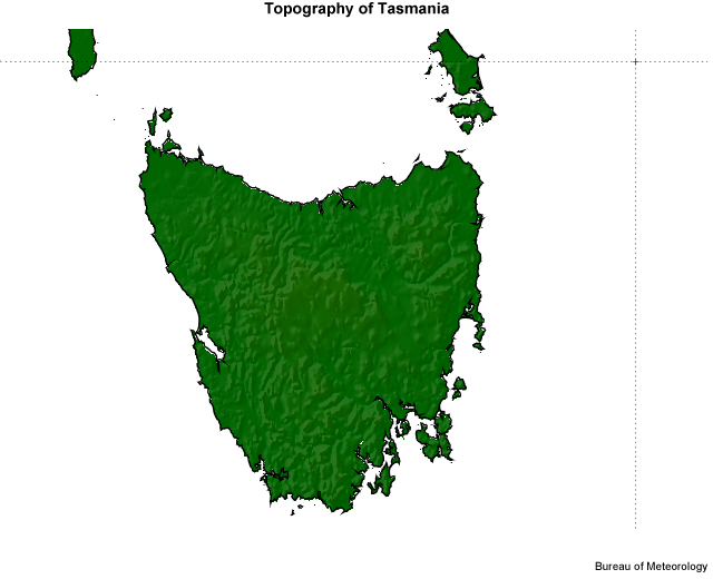
Tasmanian Case Study
Let's work through the following rain event. It occurred in October 2014 over the island of Tasmania. The island is southeast of Australia and the image below shows its topography.
Model Resolution
Examine the model rainfall fields produced by three models of various resolution.
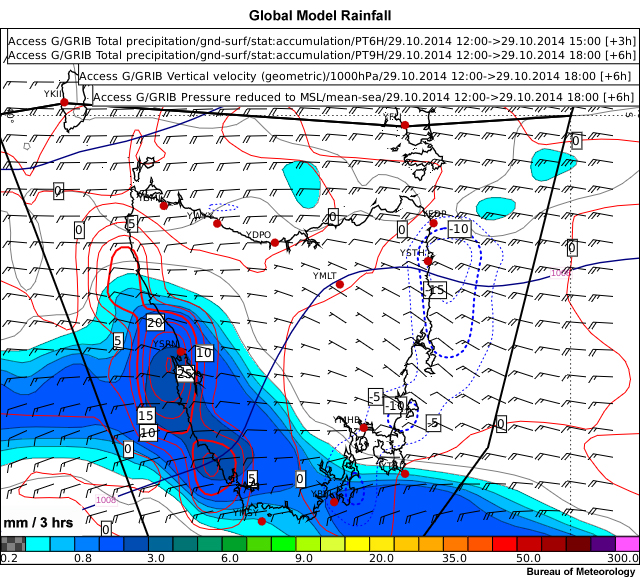
40 km Total Rainfall Content
Total rainfall, surface wind and surface vertical motion for the Bureau of Meteorology ACCESS-G global model with a horizontal resolution of ~40km.
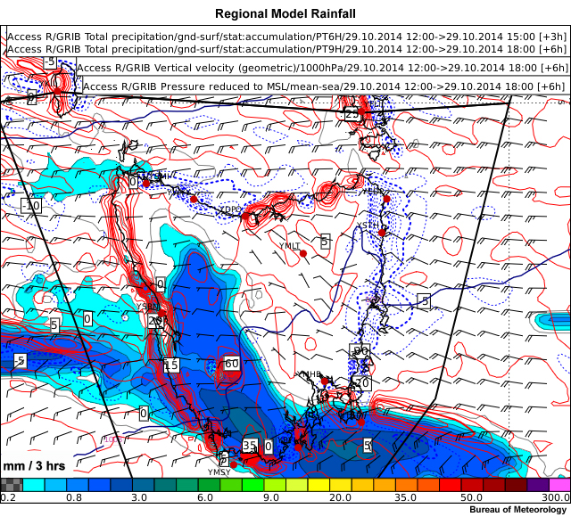
12 km total rainfall Content
Total rainfall, surface wind and surface vertical motion for the Bureau of Meteorology ACCESS-R regional model with a horizontal resolution of ~12km.
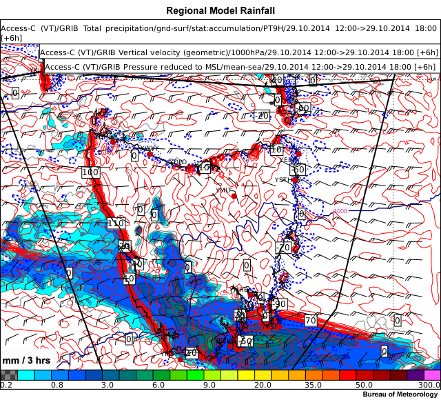
4 km total rainfall Content
Total rainfall, surface wind and surface vertical motion for the Bureau of Meteorology ACCESS-C regional model with a horizontal resolution of ~4km.
Question 1 of 2
Which region exhibits the largest changes in rainfall as model resolution increases? (Select best option)
The correct answer is b.
While there are some changes over the oceans, the land shows both a decrease in the area covered, and a shift to the west.
Question 2 of 2
What impact does the increased resolution have on the vertical motion field? (Choose all that apply.)
The correct answers are a, c.
As model resolution increases, the resolution of the horizontal wind field increases. Since ω is calculated from the continuity equation for hydrostatic models such as ACCESS, the resolution of ω will increase, which means sharper gradients and larger peak values.
Tasmanian Case Study » Wind Changes
Question 1 of 2
Using the pen tool, draw a line connecting the major wind direction changes that you see on the image.
| Tool: | Tool Size: | Color: |
|---|---|---|
|
|
The change in wind direction is well indicated over the ocean by the vertical motion field and as a wind change from west to northwest ahead and southwesterly behind the front. Over Tasmania there is a northwest to westerly wind change, which lags behind the front over the ocean, due to the topography.
In order to answer the next question, click on the white circle in the image and drag it to compare the two images. One image is from the global model ACCESS-G, the other is from the regional model ACCESS-R.
Question 2 of 2
What is the major difference between ACCESS-G and ACCESS-R in relation to the wind change?
One of the major differences between ACCESS-G and ACCESS-R is the resolving of the cold front to the southeast of Tasmania, extending through the centre of the state. In the ACCESS-G, the change is much broader and slower, lying to the west of Tasmania rather than over the land itself, but is still to the southeast over the ocean.
Tasmanian Case Study » Convective Rainfall
Continuing with the same scenario, examine the model convective rainfall fields produced by three models of various resolution.
40 km Horizontal Resolution
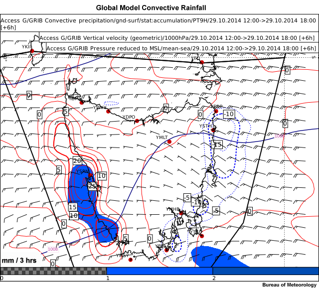
Convective rainfall, surface wind and surface vertical motion for the Bureau of Meteorology ACCESS-G global model with a horizontal resolution of ~40km.
12 km horizontal resolution
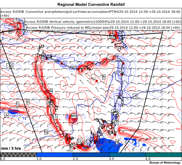
Convective rainfall, surface wind and surface vertical motion for the Bureau of Meteorology ACCESS-R regional model with a horizontal resolution of ~12km.
4 km horizontal resolution
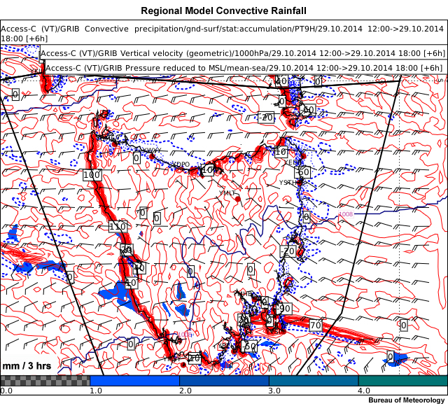
Convective rainfall, surface wind and surface vertical motion for the Bureau of Meteorology ACCESS-C regional model with a horizontal resolution of ~4km.
Question
Model convective rainfall is the indirect result of a parameterisation scheme that seeks to reduce instability in a model grid box. What happens to the convective rainfall amount as the model resolution increases? [Select best option]
The correct answer is b.
The decrease in convective rainfall is very marked in the convective rainfall field, particularly on the west coast of Tasmania. This can also be seen in the change in total rainfall field.
Tasmanian Case Study » Physical Mechanisms
Continuing with the same scenario, examine all the model guidance produced by three models of various resolution then answer the question below. Click the tabs below to select the resolution you would like to see.
40 km Total Rainfall
Total rainfall, surface wind and surface vertical motion for the Bureau of Meteorology ACCESS-G global model with a horizontal resolution of ~40km.
12 km Total Rainfall
Total rainfall, surface wind and surface vertical motion for the Bureau of Meteorology ACCESS-R regional model with a horizontal resolution of ~12km.
4 km Total Rainfall
Total rainfall, surface wind and surface vertical motion for the Bureau of Meteorology ACCESS-C regional model with a horizontal resolution of ~4km.
40 km Convective Rainfall
Convective rainfall, surface wind and surface vertical motion for the Bureau of Meteorology ACCESS-G global model with a horizontal resolution of ~40km.
12 km Convective Rainfall
Convective rainfall, surface wind and surface vertical motion for the Bureau of Meteorology ACCESS-R regional model with a horizontal resolution of ~12km.
4 km Convective Rainfall
Convective rainfall, surface wind and surface vertical motion for the Bureau of Meteorology ACCESS-C regional model with a horizontal resolution of ~4km.
Tab 3a Content
Which of the following words best describe the physical mechanisms responsible for the rainfall over Tasmania? Select all that apply.
The correct answers are b, e, f.
As model resolution increases, the convective rainfall decreases over Tasmania, so the rainfall is mostly orographic. With an increase in resolution we can also see the wind change, and most of this is in the westerly flow behind the change. Finally, the rainfall maximum appears to coincide with the ranges over Western Tasmania, indicating the role of orographic uplift.
Summary
As you have seen in this module, the "model type" affects the types of errors the model makes, and thus how to interpret the model forecast. The different ways of calculating model output and grid types influence how the models represent the structure and dynamics of the atmosphere.
In the last case, you experienced how model characteristics affected the physical characteristics and dynamics of the modeled atmospheric processes. Being aware of this and making appropriate interpretations is a crucial forecast skill that you will continue to refine over the entirety of your career as a forecaster.
Contributors
COMET Sponsors
The COMET® Program is sponsored by NOAA's National Weather Service (NWS), with additional funding by:
- Bureau of Meteorology of Australia (BoM)
- Bureau of Reclamation, United States Department of the Interior
- European Organisation for the Exploitation of Meteorological Satellites (EUMETSAT)
- Meteorological Service of Canada (MSC)
- NOAA's National Environmental Satellite, Data and Information Service (NESDIS)
- NOAA's National Geodetic Survey (NGS)
- Naval Meteorology and Oceanography Command (NMOC)
- U.S. Army Corps of Engineers (USACE)
Project Contributors
Senior Project Manager
- Bruce Muller — UCAR/COMET
Project Lead / Instructional Design
- Tsvetomir Ross-Lazarov — UCAR/COMET
- Dr. Mick Pope — Bureau of Meteorology Training Centre
Principal Science Advisors
- Dr. Mick Pope — Bureau of Meteorology Training Centre
Graphics/Animations
- Steve Deyo — UCAR/COMET
- Sylvia Quesada — UCAR/COMET
Multimedia Authoring/Interface Design
- Gary Pacheco — UCAR/COMET
- Tsvetomir Ross-Lazarov — UCAR/COMET
COMET Staff, Winter 2014
Director's Office
- Dr. Rich Jeffries, Director
- Dr. Greg Byrd, Deputy Director
- Lili Francklyn, Business Development Specialist
Business Administration
- Dr. Elizabeth Mulvihill Page, Group Manager
- Lorrie Alberta, Administrator
- Hildy Kane, Administrative Assistant
IT Services
- Tim Alberta, Group Manager
- Bob Bubon, Systems Administrator
- Dolores Kiessling, Software Engineer
- Joey Rener, Student Assistant
- Malte Winkler, Software Engineer
Instructional and Media Services
- Bruce Muller, Group Manager
- Dr. Alan Bol, Scientist/Instructional Designer
- Steve Deyo, Graphic and 3D Designer
- Lon Goldstein, Instructional Designer
- Bryan Guarente, Instructional Designer
- Vickie Johnson, Instructional Designer (Casual)
- Gary Pacheco, Web Designer and Developer
- Tsvetomir Ross-Lazarov, Instructional Designer
- David Russi, Spanish Translations
- Andrea Smith, Meteorologist/Instructional Designer
- Marianne Weingroff, Instructional Designer
Science Group
- Wendy Schreiber-Abshire, Group Manager
- Dr. William Bua, Meteorologist
- Dr. Frank Bub, Oceanographer (Casual)
- Lis Cohen, Meteorologist (Casual)
- Patrick Dills, Meteorologist
- Matthew Kelsch, Hydrometeorologist
- Nicolas Major, Visiting Meteorologist, Meteorological Services of Canada
- Dr. Elizabeth Mulvihill Page, Meteorologist
- Amy Stevermer, Meteorologist
- Vanessa Vincente, Visiting Meteorologist, CIRA/Colorado State University